1. Vectors ベクトル

1.1 Definitions (basic) (基本)定義

There are many ways to define a vector. For starters, here's the most basic:
ベクトルを定義する方法はたくさんあります。まずは最も基本的な方法をご紹介します。

A vector is the mathematical representation of a physical entity that may be characterized by size (or “magnitude”) and direction.
ベクトルは、サイズ (または「大きさ」) と方向によって特徴付けられる物理的実体の数学的表現です。

In keeping with this definition, speed (how fast an object is going) is not represented by a vector, but velocity (how fast and in which direction an object is going) does qualify as a vector quantity. Another example of a vector quantity is force, which describes how strongly and in what direction something is being pushed or pulled. But temperature, which has magnitude but no direction, is not a vector quantity.
この定義に従うと、スピード（速さ。物体がどれだけ速く動いているか）はベクトルで表されませんが、速度（物体がどれだけ速く、どの方向に動いているか）はベクトル量として扱われます。ベクトル量のもう一つの例は力です。力は、物体がどれだけ強く、どの方向に押されたり引っ張られたりするかを記述します。しかし、温度は大きさはあっても方向がないため、ベクトル量ではありません。

The word “vector” comes from the Latin vehere meaning “to carry;” it was first used by eighteenth-century astronomers investigating the mechanism by which a planet is “carried” around the Sun.¹ In text, the vector nature of an object is often indicated by placing a small arrow over the variable representing the object (such as \(\vec{F}\)), or by using a bold font (such as \(\mathbf{F}\)), or by underlining (such as \(\underline{F}\) or \(\underset{\sim}{F}\) ). When you begin hand-writing equations involving vectors, it's very important that you get into the habit of denoting vectors using one of these techniques (or another one of your choosing). The important thing is not how you denote vectors, it's that you don't simply write them the same way you write non-vector quantities.

¹ The Oxford English Dictionary. 2nd ed. 1989.

「ベクトル」という単語は、ラテン語の「運ぶ」という意味の vehere に由来します。この単語が最初に使われたのは、惑星が太陽の周りを「運ばれる」メカニズムを調査していた 18 世紀の天文学者です。¹ テキストでは、オブジェクトのベクトルの性質は、多くの場合、オブジェクトを表す変数の上に小さな矢印を付けたり (\(\vec{F}\) など)、太字のフォントを使用したり (\(\mathbf{F}\) など)、下線を引いたり (\(\underline{F}\) または \(\underset{\sim}{F}\) など) することで示されます。ベクトルを含む数式を手書きで書き始めるときは、これらの技法 (または別の選択した技法) のいずれかを使用してベクトルを表す習慣を身に付けることが非常に重要です。重要なのは、ベクトルをどのように表すかではなく、非ベクトル量と同じように単純に書かないことです。

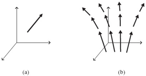
A vector is most commonly depicted graphically as a directed line segment or an arrow, as shown in Figure 1.1(a). And as you'll see later in this section, a vector may also be represented by an ordered set of N numbers, where N is the number of dimensions in the space in which the vector resides.
ベクトルは、図1.1(a)に示すように、有向線分または矢印として図的に表されるのが最も一般的です。また、このセクションの後半で説明するように、ベクトルはN個の数値の順序付き集合で表すこともできます。ここで、Nはベクトルが存在する空間の次元数です。

Of course, the true value of a vector comes from knowing what it represents. The vector in Figure 1.1(a), for example, may represent the velocity of the wind at some location, the acceleration of a rocket, the force on a football, or any of the thousands of vector quantities that you encounter in the world every day. Whatever else you may learn about vectors, you can be sure that every one of them has two things: size and direction. The magnitude of a vector is usually indicated by the length of the arrow, and it tells you the amount of the quantity represented by the vector. The scale is up to you (or whoever's drawing the vector), but once the scale has been established, all other vectors should be drawn to the same scale. Once you know that scale, you can determine the magnitude of any vector just by finding its length. The direction of the vector is usually given by indicating the angle between the arrow and one or more specified directions (usually the “coordinate axes”), and it tells you which way the vector is pointing.
もちろん、ベクトルの真の価値は、それが何を表しているかを知ることから生まれます。例えば、図 1.1(a) のベクトルは、ある場所における風速、ロケットの加速度、フットボールにかかる力、あるいは日々の世界で目にする何千ものベクトル量を表しているかもしれません。ベクトルについて何を学んだとしても、すべてのベクトルには大きさと方向という2つの要素があることは間違いありません。ベクトルの大きさは通常、矢印の長さで示され、ベクトルが表す量の量を示します。スケールはあなた（またはベクトルを描く人）次第ですが、一度スケールが確立されれば、他のすべてのベクトルは同じスケールで描く必要があります。スケールがわかれば、ベクトルの長さを求めるだけで大きさを判断できます。ベクトルの方向は通常、矢印と1つまたは複数の指定された方向（通常は「座標軸」）との間の角度を示すことで示され、ベクトルがどの方向を向いているかを示します。

So if vectors are characterized by their magnitude and direction, does that mean that two equally long vectors pointing in the same direction could in fact be considered to be the same vector? In other words, if you were to move the vector shown in Figure 1.1(a) to a different location without varying its length or its pointing direction, would it still be the same vector? In some applications, the answer is “yes,” and those vectors are called free vectors. You can move a free vector anywhere you'd like as long as you don't change its length or direction, and it remains the same vector. But in many physics and engineering problems, you'll be dealing with vectors that apply at a given location; such vectors are called “bound” or “anchored” vectors, and you're not allowed to relocate bound vectors as you can free vectors.² You may see the term “sliding” vectors used for vectors that are free to move along their length but are not free to change length or direction; such vectors are useful for problems involving torque and angular motion.
では、ベクトルが大きさと方向によって特徴付けられるのであれば、同じ方向を向いている等しい長さのベクトル 2 つは、実際には同じベクトルと見なせるのでしょうか。言い換えれば、図 1.1(a) に示されているベクトルを、長さや向きを変えずに別の場所に移動した場合、それでも同じベクトルになるのでしょうか。アプリケーションによっては、答えは「はい」であり、そのようなベクトルは自由ベクトルと呼ばれます。自由ベクトルは、長さや向きを変えない限り、どこにでも移動でき、同じベクトルのままです。しかし、多くの物理学や工学の問題では、特定の場所に適用されるベクトルを扱います。このようなベクトルは「拘束」ベクトルまたは「固定」ベクトルと呼ばれ、自由ベクトルのように拘束ベクトルを再配置することはできません。² 長さに沿って自由に移動できるが、長さや方向を自由に変更できないベクトルに対して、「スライディング」ベクトルという用語が使用されることがあります。このようなベクトルは、トルクや角運動を含む問題に役立ちます。

² Mathematicians don't have much use for bound vectors, since the mathematical definition of a vector deals with how it transforms rather than where it's located.
ベクトルの数学的定義は、ベクトルがどこに位置するかではなく、ベクトルがどのように変換されるかを扱うため、数学者は境界ベクトルをあまり使用しません。

You can understand the usefulness of bound vectors if you think about an application such as representing the velocity of the wind at various points in the atmosphere. To do that, you could choose to draw a bound vector at each point of interest, and each of those vectors would show the speed and direction of the wind at that location (most people draw the vector with its tail – the end without the arrow – at the point to which the vector is bound). A collection of such vectors is called a vector field; an example is shown in Figure 1.1(b).
大気中の様々な地点における風速を表すような応用を考えれば、境界ベクトルの有用性は理解できるでしょう。例えば、関心のある各地点に境界ベクトルを描くと、それぞれのベクトルがその地点における風速と風向を示します（多くの人は、ベクトルの尾（矢印のない端）を、ベクトルが境界となる地点に沿わせて描きます）。このようなベクトルの集合はベクトル場と呼ばれます。図1.1(b)に例を示します。

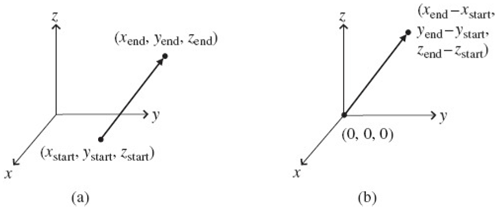
If you think about the ways in which you might represent a bound vector, you may realize that the vector can be defined simply by specifying the start and end points of the arrow. So in a three-dimensional Cartesian coordinate system, you only need to know the values of x, y, and z for each end of the vector, as shown in Figure 1.2(a) (you can read about vector representation in non-Cartesian coordinate systems later in this chapter).
境界ベクトルの表現方法を考えてみると、矢印の始点と終点を指定するだけでベクトルを定義できることに気づくでしょう。つまり、3次元直交座標系では、図1.2(a)に示すように、ベクトルの両端のx、y、zの値さえ分かれば十分です（非直交座標系におけるベクトル表現については、この章の後半で説明します）。

Now consider the special case in which the vector is anchored to the origin of the coordinate system (that is, the end without the arrowhead is at the point of intersection of the coordinate axes, as shown in Figure 1.2(b).³ Such vectors may be completely specified simply by listing the three numbers that represent the x-, y-, and z-coordinates of the vector's end point. Hence a vector anchored to the origin and stretching five units along the x-axis may be represented as (5,0,0). In this representation, the values that represent the vector are called the “components” of the vector, and the number of components it takes to define a vector is equal to the number of dimensions in the space in which the vector exists. So in a two-dimensional space a vector may be represented by a pair of numbers, and in four-dimensional spacetime vectors may appear as lists of four numbers. This explains why a horizontal list of numbers is called a “row vector” and a vertical list of numbers is called a “column vector” in computer science. The number of values in such vectors tells you how many dimensions there are in the space in which the vector resides.
ここで、ベクトルが座標系の原点に固定されている（つまり、矢印のない端が座標軸の交点にある）特殊なケースを考えてみましょう（図 1.2(b)³ に示すように）。このようなベクトルは、ベクトルの終点の x、y、z 座標を表す 3 つの数値をリストするだけで完全に指定できます。したがって、原点に固定され、x 軸に沿って 5 単位伸びるベクトルは、(5,0,0) と表すことができます。この表現では、ベクトルを表す値はベクトルの「成分」と呼ばれ、ベクトルを定義するために必要な成分の数は、ベクトルが存在する空間の次元数に等しくなります。したがって、2 次元空間ではベクトルは 2 つの数値で表され、4 次元時空ではベクトルは 4 つの数値のリストとして現れることがあります。これが、コンピュータ サイエンスで水平方向の数値リストを「行ベクトル」、垂直方向の数値リストを「列ベクトル」と呼ぶ理由です。このようなベクトルの値の数は、ベクトルは、ベクトルが存在する空間にいくつの次元があるかを示します。

³ The vector shown in Figure 1.2 (a) can be shifted to this location by subtracting xstart, ystart, and zstart from the values at each end.
図 1.2 (a) に示すベクトルは、各端の値から xstart、ystart、zstart を減算することで、この位置に移動できます。

To understand how vectors are different from other entities, it may help to consider the nature of some things that are clearly not vectors. Think about the temperature in the room in which you're sitting – at each point in the room, the temperature has a value, which you can represent by a single number. That value may well be different from the value at other locations, but at any given point the temperature can be represented by a single number, the magnitude. Such magnitude-only quantities have been called “scalars” ever since W.R. Hamilton referred to them as “all values contained on the one scale of progression of numbers from negative to positive infinity.”⁴ Thus
ベクトルが他の実体とどのように異なるかを理解するには、明らかにベクトルではないものの性質について考えてみると役立つかもしれません。あなたが座っている部屋の温度について考えてみましょう。部屋の各点の温度は値を持ち、単一の数値で表すことができます。その値は他の場所の値とは異なる場合がありますが、任意の点の温度は単一の数値、つまり大きさで表すことができます。このような大きさのみを持つ量は、W.R.ハミルトンが「負の無限大から正の無限大までの数の進行の単一のスケールに含まれるすべての値」と呼んで以来、「スカラー」と呼ばれています。⁴ つまり、

⁴ W.R. Hamilton, Phil. Mag. XXIX, 26.

A scalar is the mathematical representation of a physical entity that may be characterized by magnitude only.
スカラーは、大きさのみで特徴付けられる物理的実体の数学的表現です。

Other examples of scalar quantities include mass, charge, energy, and speed (defined as the magnitude of the velocity vector). It is worth noting that the change in temperature over a region of space does have both magnitude and direction and may therefore be represented by a vector, so it's possible to produce vectors from groups of scalars. You can read about just such a vector (called the “gradient” of a scalar field) in Chapter 2.
スカラー量の他の例としては、質量、電荷、エネルギー、速度（速度ベクトルの大きさとして定義されます）などがあります。注目すべきは、空間領域における温度変化は大きさと方向の両方を持ち、ベクトルで表すことができるということです。つまり、スカラーの集合からベクトルを生成することが可能です。このようなベクトル（スカラー場の「勾配」と呼ばれます）については、第2章で説明します。

Since scalars can be represented by magnitude only (single numbers) and vectors by magnitude and direction (three numbers in three-dimensional space), you might suspect that there are other entities involving magnitude and directions that are more complex than vectors (that is, requiring more numbers than the number of spatial dimensions). Indeed there are, and such entities are called “tensors.”⁵ You can read about tensors in the last three chapters of this book, but for now this simple definition will suffice:
スカラーは大きさ（単一の数値）のみで表すことができ、ベクトルは大きさと方向（3次元空間における3つの数値）で表すことができるため、ベクトルよりも複雑な（つまり、空間の次元数よりも多くの数値を必要とする）大きさと方向を含む実体が存在するのではないかと考えるかもしれません。確かにそのような実体は存在し、そのような実体は「テンソル」と呼ばれます。⁵ テンソルについては本書の最後の3章で解説しますが、今はこの簡単な定義で十分でしょう。

⁵ As you can learn in the later portions of this book, scalars and vectors also belong to the class of objects called tensors but have lower rank, so in this section the word “tensors” refers to higher-rank tensors.
この本の後半で学習するように、スカラーとベクトルもテンソルと呼ばれるオブジェクトのクラスに属しますが、ランクが低いため、このセクションでは「テンソル」という語は高ランクのテンソルを指します。

A tensor is the mathematical representation of a physical entity that may be characterized by magnitude and multiple directions.
テンソルは、大きさと複数の方向によって特徴付けられる物理的実体の数学的表現です。

An example of a tensor is the inertia that relates the angular velocity of a rotating object to its angular momentum. Since the angular velocity vector has a direction and the angular momentum vector has a (potentially different) direction, the inertia tensor involves multiple directions.
テンソルの一例としては、回転する物体の角速度と角運動量を関連付ける慣性が挙げられます。角速度ベクトルには方向があり、角運動量ベクトルには（場合によっては異なる）方向があるため、慣性テンソルは複数の方向を包含します。

And just as a scalar may be represented by a single number and a vector may be represented by a sequence of three numbers in 3-dimensional space, a tensor may be represented by an array of 3R numbers in 3-dimensional space. In this expression, “R” represents the rank of the tensor. So in 3-dimensional space, a second-rank tensor is represented by 32 = 9 numbers. In N-dimensional space, scalars still require only one number, vectors require N numbers, and tensors require NR numbers.
3次元空間において、スカラーが単一の数値で表され、ベクトルが3つの数値の列で表されるように、テンソルは3次元空間において3R個の数値の配列で表されます。この式で、「R」はテンソルの階数を表します。つまり、3次元空間では、2階テンソルは32 = 9個の数値で表されます。N次元空間では、スカラーは依然として1個の数値で表され、ベクトルはN個の数値、テンソルはNR個の数値で表されます。

Recognizing scalars, vectors, and tensors is easy once you realize that a scalar can be represented by a single number, a vector by an ordered set of numbers, and a tensor by an array of numbers. So in three-dimensional space, they look like this:
スカラー、ベクトル、テンソルは、スカラーが単一の数値、ベクトルが順序付けられた数値の集合、テンソルが数値の配列で表せることを理解すれば、簡単に理解できます。3次元空間では、これらは次のようになります。 \[ \begin{array}{c c c} \underline{Scalar} & \underline{Vector} & \underline{Tensor (Rank 2)} \\ (x) & (x_1,x_2,x_3)\;or\;\begin{pmatrix} x_1 \\ x_2\\ x_3 \end{pmatrix} & \begin{pmatrix} x_{11} & x_{12} & x_{13} \\ x_{21} & x_{22} & x_{23} \\ x_{31} & x_{32} & x_{33} \end{pmatrix} \end{array} \]

Note that scalars require no subscripts, vectors require a single subscript, and tensors require two or more subscripts – the tensor shown here is a tensor of rank 2, but you may also encounter higher-rank tensors, as discussed in Chapter 5. A tensor of rank 3 may be represented by a three-dimensional array of values.
スカラーには添字は必要なく、ベクトルには 1 つの添字が必要ですが、テンソルには 2 つ以上の添字が必要であることに注意してください。ここで示されているテンソルは階数 2 のテンソルですが、第 5 章で説明されているように、より高階数のテンソルに遭遇することもあります。階数 3 のテンソルは、値の 3 次元配列で表すことができます。

With these basic definitions in hand, you're ready to begin considering the ways in which vectors can be put to use. Among the most useful of all vectors are the Cartesian unit vectors, which you can read about in the next section.
これらの基本的な定義を理解したら、ベクトルの活用方法を考え始める準備が整いました。ベクトルの中でも最も有用なものの一つが直交座標単位ベクトルです。これについては次のセクションで説明します。

1.2 Cartesian unit vectors デカルト座標単位ベクトル

If you hope to use vectors to solve problems, it's essential that you learn how to handle situations involving more than one vector. The first step in that process is to understand the meaning of special vectors called “unit vectors” that often serve as markers for various directions of interest (unit vectors may also be called “versors”).
ベクトルを使って問題を解きたい場合、複数のベクトルが関わる状況への対処法を学ぶことが不可欠です。その第一歩は、「単位ベクトル」と呼ばれる特殊なベクトルの意味を理解することです。単位ベクトルは、様々な方向を示すマーカーとしてよく使用されます（単位ベクトルは「バーサー」と呼ばれることもあります）。

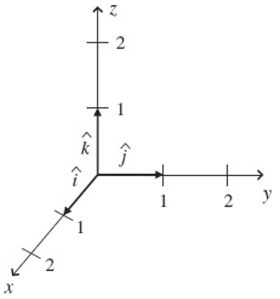
The first unit vectors you're likely to encounter are the unit vectors \(\hat{x},\hat{y},\hat{z}\) (also called \(\hat{i},\hat{j},\hat{k}\)) that point in the direction of the \(x\)-, \(y\)-, and \(z\)-axes of the three- dimensional Cartesian coordinate system, as shown in Figure 1.3. These vectors are called unit vectors because their length (or magnitude) is always exactly equal to unity, which is another name for “one.” One what? One of whatever units you're using for that axis.
おそらく最初に遭遇する単位ベクトルは、図 1.3 に示すように、3 次元直交座標系の \(x\) 軸、\(y\) 軸、\(z\) 軸の方向を指す単位ベクトル \(\hat{x},\hat{y},\hat{z}\) (または \(\hat{i},\hat{j},\hat{k}\) とも呼ばれます) です。これらのベクトルは、その長さ (または大きさ) が常に 1 (「1」の別名) と正確に等しいため、単位ベクトルと呼ばれます。1 とは何でしょうか? その軸に使用している単位の 1 つです。

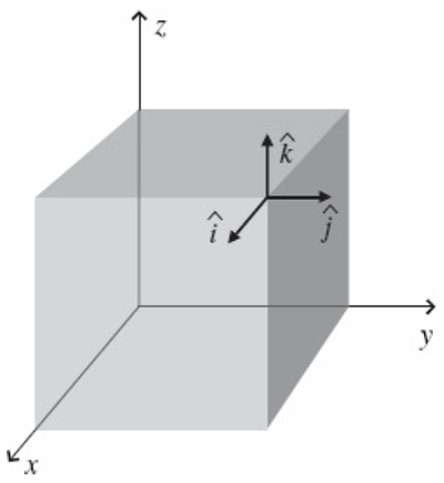
You should note that the Cartesian unit vectors \(\hat{i},\hat{j},\hat{k}\) can be drawn at any location, not just at the origin of the coordinate system. This is illustrated in Figure 1.4. As long as you draw a vector of unit length pointing in the same direction as the direction of the (increasing) \(x\)-axis, you've drawn the \(\hat{i}\) unit vector. So the Cartesian unit vectors show you the directions of the \(x, y,\) and \(z\) axes, not the location of the origin.
直交座標の単位ベクトル \(\hat{i},\hat{j},\hat{k}\) は、座標系の原点だけでなく、任意の位置に描くことができることに注意してください。これは図1.4に示されています。\(x\)軸（増加する）の方向と同じ方向を指す単位長さのベクトルを描けば、\(\hat{i}\) 単位ベクトルを描いたことになります。つまり、直交座標の単位ベクトルは、原点の位置ではなく、\(x, y,\)軸と\(z\)軸の方向を示します。

As you'll see in Chapter 2, unit vectors can be extremely helpful when doing certain operations such as specifying the portion of a given vector pointing in a certain direction. That's because unit vectors don't have their own magnitude to throw into the mix (actually, they do have their own magnitude, but it is always one).
第2章で解説するように、単位ベクトルは、あるベクトルのどの部分が特定の方向を指すかを指定するといった特定の操作を行う際に非常に役立ちます。これは、単位ベクトルには独自の大きさがないため（実際には独自の大きさはありますが、常に1です）、ベクトルの向きを計算に組み込む必要がないためです。

So when you see an expression such as “\(5\hat{i},\)” you should think “5 units along the positive \(x\)-direction.” Likewise, \(–3\hat{j}\) refers to 3 units along the negative \(y\)- direction, and \(\hat{k}\) indicates one unit along the positive \(z\)-direction.
したがって、「\(5\hat{i},\)」のような表現を見たら、「正の\(x\)方向に沿って5単位」と考えるべきです。同様に、\(–3\hat{j}\)は負の\(y\)方向に沿って3単位を指し、\(\hat{k}\)は正の\(z\)方向に沿って1単位を示します。

Of course, there are other coordinate systems in addition to the three perpendicular axes of the Cartesian system, and unit vectors exist in those coordinate systems as well; you can see some examples in Section 1.5. One advantage of the Cartesian unit vectors is that they point in the same direction no matter where you go; the \(x\)-, \(y\)-, and \(z\)-axes run in straight lines all the way out to infinity, and the Cartesian unit vectors are parallel to the directions of those lines everywhere.
もちろん、直交座標系の3つの直交軸以外にも座標系は存在し、それらの座標系にも単位ベクトルが存在します。セクション1.5でいくつかの例を見ることができます。直交座標系単位ベクトルの利点の一つは、どこに行っても同じ方向を向いていることです。\(x\)軸、\(y\)軸、\(z\)軸は無限遠まで直線状に伸びており、直交座標系単位ベクトルはどの位置においてもこれらの直線の方向と平行です。

To put unit vectors such as \(\hat{i},\hat{j},\hat{k}\) to work, you need to understand the concept of vector components. The next section shows you how to represent vectors using unit vectors and vector components.
\(\hat{i},\hat{j},\hat{k}\) のような単位ベクトルを使うには、ベクトル成分の概念を理解する必要があります。次のセクションでは、単位ベクトルとベクトル成分を用いてベクトルを表現する方法を説明します。

1.3 Vector components ベクトル成分

The unit vectors described in the previous section are especially useful when they become part of the “components” of a vector. And what are the components of a vector? Simply stated, they are the pieces that can be used to make up the vector.
前のセクションで説明した単位ベクトルは、ベクトルの「成分」の一部となると特に便利です。では、ベクトルの成分とは何でしょうか？簡単に言えば、ベクトルを構成する要素のことです。

To understand vector components, think about the vector \(\vec{A}\) shown in Figure 1.5. This is a bound vector, anchored at the origin and extending to the point (\(x = 0, y = 3, z = 3\)) in a three-dimensional Cartesian coordinate system. So if you consider the coordinate axes as representing the corner of a room, this vector is embedded in the back wall (the \(yz\) plane).
ベクトル成分を理解するには、図1.5に示すベクトル\(\vec{A}\)について考えてみましょう。これは、原点を基準として、3次元直交座標系の点(\(x = 0, y = 3, z = 3\))まで伸びる境界ベクトルです。つまり、座標軸を部屋の角を表すものと見なすと、このベクトルは奥の壁（\(yz\)平面）に埋め込まれていることになります。

Imagine you're trying to get from the beginning of vector \(\vec{A}\) to the end – the direct route would be simply to move in the direction of the vector. But if you were constrained to move only in the directions of the axes, you could get from the origin to your destination by taking three (unit) steps along the y-axis, then turning 90° to your left, and then taking three more (unit) steps in the direction of the \(z\)-axis.
ベクトル \(\vec{A}\) の始点から終点まで移動しようとしていると想像してください。直線的な経路は、ベクトルの方向に移動するだけです。しかし、軸方向にのみ移動するように制約されている場合、y軸方向に3（単位）ステップ移動し、左に90°回転し、さらに \(z\) 軸方向に3（単位）ステップ移動することで、原点から目的地まで移動できます。

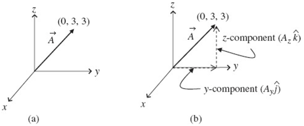
What does this little journey have to do with the components of a vector? Simply this: the lengths of the components of vector \(\vec{A}\) are the distances you traveled in the directions of the axes. Specifically, in this case the magnitude of the \(y\)-component of vector \(\vec{A}\) (written as \(A_y\)) is just the distance you traveled in the direction of the \(y\)-axis (3 units), and the magnitude of the \(z\)-component of vector \(\vec{A}\) (written as \(A_z\)) is the distance you traveled in the direction of the \(z\)-axis (also 3 units). Since you didn't move at all in the direction of the \(x\)-axis, the magnitude of the \(x\)-component of vector \(\vec{A}\) (written as \(A_x\)) is zero.
このちょっとした旅は、ベクトルの成分とどのような関係があるのでしょうか？簡単に言うと、ベクトル \(\vec{A}\) の成分の長さは、軸方向に移動した距離です。具体的には、この場合、ベクトル \(\vec{A}\) の \(y\) 成分（\(A_y\) と表記）の大きさは、\(y\) 軸方向に移動した距離（3単位）であり、ベクトル \(\vec{A}\) の \(z\) 成分（\(A_z\) と表記）の大きさは、\(z\) 軸方向に移動した距離（これも3単位）です。 \(x\) 軸方向にはまったく移動していないため、ベクトル \(\vec{A}\) (\(A_x\) と表記) の \(x\) 成分の大きさはゼロになります。

A very handy and compact way of writing a vector as a combination of vector components is this:
ベクトルをベクトル要素の組み合わせとして記述する非常に便利でコンパクトな方法は次のとおりです。 \[ \vec{A} = A_x\hat{i}+A_y\hat{j}+A_z\hat{k} \tag{1.1} \] where the magnitudes of the vector components (\(A_x, A_y,\) and \(A_z\)) tell you how many unit steps to take in each direction (\(\hat{i},\hat{j},\) and \(\hat{k}\)) to get from the beginning to the end of vector \(\vec{A}\).⁶
ここで、ベクトル成分 (\(A_x, A_y,\)、\(A_z\)) の大きさは、ベクトル \(\vec{A}\) の先頭から末尾まで到達するために各方向 (\(\hat{i},\hat{j},\)、\(\hat{k}\)) に何単位ステップ進む必要があるかを示します。⁶

⁶ Some authors refer to the magnitudes Ax, Ay, and Az as the “components of ,” while others consider the components to be Axî, Ay ĵ, and Az . Just remember that Ax, Ay, and Az are scalars, but Axî, Ay ĵ, and Az are vectors.
著者によっては、Ax、Ay、Az の大きさを「 の成分」と呼ぶ人もいますが、Axî、Ayĵ、Az と考える人もいます。Ax、Ay、Az はスカラーですが、Axî、Ayĵ、Az はベクトルであることを覚えておいてください。

When you read about vectors and vector components, you're likely to run across statements such as “The components of a vector are the projections of the vector onto the coordinate axes.” As you can see in Chapter 4, exactly how those projections are made can have a significant influence on the nature of the components you get. But in Cartesian coordinate systems (and other “orthogonal” systems in which the axes are perpendicular to one another), the concept of projection onto the coordinate axes is unambiguous and may be very helpful in picturing the components of a vector.
ベクトルとベクトル成分について読むと、「ベクトルの成分は、ベクトルを座標軸に投影したものである」といった記述に遭遇するでしょう。第4章でわかるように、これらの投影がどのように行われるかは、得られる成分の性質に大きな影響を与える可能性があります。しかし、直交座標系（および軸が互いに直交するその他の「直交」座標系）では、座標軸への投影の概念は明確であり、ベクトルの成分を視覚的に理解するのに非常に役立ちます。

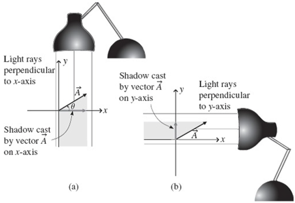
To understand how this works, take a look at vector \(\vec{A}\) and the light sources and shadows in Figure 1.6. As you can see in Figure 1.6(a), the direction of the light that produces the shadow on the \(x\)-axis is parallel to the y-axis (actually antiparallel since it's moving in the negative y-direction), which in this case is the same as saying that the direction of the light is perpendicular to the x-axis.
この仕組みを理解するには、図1.6のベクトル\(\vec{A}\)と光源、そして影を見てください。図1.6(a)に示すように、\(x\)軸上に影を生み出す光の方向はy軸と平行です（実際にはy軸の負の方向に動いているため、反平行です）。この場合、光の方向はx軸に垂直であるのと同じです。

Likewise, in Figure 1.6(b), the direction of the light that produces the shadow on the \(y\)-axis is antiparallel to the \(x\)-axis, which is of course perpendicular to the \(y\)-axis. This may seem like a trivial point, but when you encounter non- orthogonal coordinate systems, you'll find that the direction parallel to one axis is not necessarily perpendicular to another axis, which gives rise to an entirely different type of vector component. This simple fact has profound implications for the behavior of vectors and tensors for observers in different reference frames, as you'll see in Chapters 4, 5, and 6.
同様に、図1.6(b)では、\(y\)軸上に影を生み出す光の方向は\(x\)軸と反平行であり、\(x\)軸は当然\(y\)軸に垂直です。これは些細なことのように思えるかもしれませんが、非直交座標系を扱う場合、ある軸に平行な方向が必ずしも別の軸に垂直であるとは限らないことに気づきます。これにより、全く異なる種類のベクトル成分が生じます。この単純な事実は、第4章、第5章、第6章で説明するように、異なる座標系における観測者のベクトルとテンソルの挙動に深い意味を持ちます。

No such issues arise in the two-dimensional Cartesian coordinate system shown in Figure 1.6, and in this case the magnitudes of the components of vector \(\vec{A}\) are easy to determine. If the angle between vector \(vec{A}\) and the positive \(x\)-axis is \(θ\), as shown in Figure 1.6a, it's clear that the length of \(\vec{A}\) can be seen as the hypotenuse of a right triangle. The sides of that triangle along the \(x\)- and \(y\)-axes are the components Ax and Ay. Hence by simple trigonometry you can write:
図1.6に示す2次元直交座標系では、このような問題は発生せず、この場合、ベクトル\(\vec{A}\)の成分の大きさは簡単に決定できます。図1.6aに示すように、ベクトル\(vec{A}\)と\(x\)軸正方向との間の角度が\(θ\)である場合、\(\vec{A}\)の長さは直角三角形の斜辺と見なせることは明らかです。この三角形の\(x\)軸と\(y\)軸に沿った辺は、成分AxとAyです。したがって、簡単な三角法で次のように書けます。 \[ \begin{align} A_x &=|\vec{A}|\cos(\theta) \\ \\ A_y &= |\vec{A}|\sin(\theta) \end{align} \tag{1.2} \] where the vertical bars on each side of \(\vec{A}\) signify the magnitude (length) of vector \(\vec{A}\). Notice that so long as you measure the angle \(θ\) from the positive \(x\)-axis in the direction toward the positive \(y\)-axis (that is, counterclockwise in this case), these equations will give the correct sign for the \(x\)- and \(y\)-components no matter which quadrant the vector occupies.
ここで、\(\vec{A}\) の両側にある縦棒は、ベクトル \(\vec{A}\) の大きさ（長さ）を表します。\(θ\) の角度を、\(x\) 軸の正方向から \(y\) 軸の正方向（つまり、この場合は反時計回り）に測定する限り、ベクトルがどの象限に位置していても、これらの式は \(x\) 成分と \(y\) 成分の正しい符号を与えます。

For example, if vector \(\vec{A}\) is a vector with a length of 7 meters pointing in a direction 210° counter-clockwise from the \(+x\)-axis, the \(x\)- and \(y\)-components are given by Eq. 1.2 as
例えば、ベクトル\(\vec{A}\)が\(+x\)軸から反時計回りに210°の方向を指す長さ7メートルのベクトルである場合、\(x\)成分と\(y\)成分は式1.2で次のように表されます。 \[ \begin{align} Ax &= |\vec{A}|\cos(θ) = 7m \cos 210^\circ = –6.1 m \\ \\ Ay &= |\vec{A}|\sin(θ) = 7m \sin 210^\circ = –3.5m \end{align} \tag{1.3} \] As expected for a vector pointing down and to the left from the origin, both components are negative.
原点から下向きかつ左向きのベクトルの場合、両方の要素は負になります。

It's equally straightforward to find the length and direction of a vector if you're given the vector's Cartesian components. Since the vector forms the hypotenuse of a right triangle with sides \(A_x\) and \(A_y\), the Pythagorean theorem tells you that the length of \(\vec{A}\) must be
ベクトルの長さと方向は、ベクトルの直交座標成分が与えられていれば、同じように簡単に求めることができます。ベクトルは、辺\(A_x\)と\(A_y\)を持つ直角三角形の斜辺を形成するため、ピタゴラスの定理によれば、\(\vec{A}\)の長さは次の式で表されます。 \[ |\vec{A}| = \sqrt{A_x^2+A_y^2} \tag{1.4} \] and from trigonometry
そして三角法から \[ \theta = \arctan\left(\frac{A_y}{A_x}\right) \tag{1.5} \] where \(θ\) is measured counter-clockwise from the positive \(x\)-axis in a right- handed coordinate system. If you try this with the components of vector \(\vec{A}\) from Eq. 1.3 and end up with a direction of 30° rather than 210°, remember that unless you have a four-quadrant arctan function on your calculator, you must add 180° to the angle whenever the denominator of the expression (\(A_x\) in this case) is negative.
ここで、\(θ\)は右手座標系において、正の\(x\)軸から反時計回りに測られます。式1.3のベクトル\(\vec{A}\)の成分でこれを試して、210°ではなく30°の方向になった場合、電卓に4象限逆正接関数がない限り、式の分母（この場合は\(A_x\)）が負の場合は常に角度に180°を加算する必要があることに注意してください。

Once you have a working understanding of unit vectors and vector components, you're ready to do basic vector operations. The entirety of Chapter 2 is devoted to such operations, but two of them are needed for the remainder of this chapter. For that reason, you can read about vector addition and multiplication by a scalar in the next section.
単位ベクトルとベクトル成分について実用的な理解ができたら、基本的なベクトル演算を行う準備が整います。第2章全体はこれらの演算に費やされていますが、そのうち2つは本章の残りの部分で必要になります。そのため、次のセクションではベクトルの加算とスカラーによる乗算について学習します。

1.4 Vector addition and multiplication by a scalar ベクトルの加算とスカラーによる乗算

If you've read the previous section on vector components, you've already seen two vector operations in action. Those two operations are the addition of vectors and multiplication of a vector by a scalar. Both of these operations are used in the expansion of a vector in terms of vector components as in Eq. 1.1 from Section 1.3:
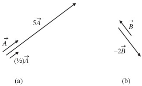
ベクトル成分に関する前のセクションを読んだ方は、既に2つのベクトル演算についてご覧になっていると思います。その2つの演算とは、ベクトルの加算とベクトルとスカラーの乗算です。これらの演算はどちらも、セクション1.3の式1.1に示すように、ベクトルをベクトル成分で展開する際に用いられます。 \[ \vec{A}=A_x\hat{i}+A_y\hat{j}+A_z\hat{k} \] In each of these terms, the unit vector (\(\hat{i},\hat{j},\) or \(\hat{k}\)) is being multiplied by a scalar (\(A_x, A_y,\) or \(A_z\)), and you already know the effect of that: it produces a new vector, in the same direction as the unit vector, but longer than unity by the value of the component (or shorter if the magnitude of the component is between zero and one). So multiplying a vector by any positive scalar does not change the direction of the vector, but only scales the length of the vector. Hence, \(5\vec{A}\) is a vector in exactly the same direction as \(\vec{A}\), but with length five \(\vec{A}\), as shown in Figure 1.7(a). Likewise, multiplying \(\vec{A}\) by (1/2) produces a vector that points in the same direction as \(\vec{A}\) but is only half as long. So the vector component \(A_x\hat{i}\) is a vector in the \(\hat{i}\) direction, but with length \(A_x\) units (since \(\hat{i}\) has a length of one unit).
これらの各項では、単位ベクトル (\(\hat{i},\hat{j},\) または \(\hat{k}\)) にスカラー (\(A_x, A_y,\) または \(A_z\)) が乗算されており、その効果は既にご存じのとおりです。つまり、単位ベクトルと同じ方向の新しいベクトルが生成されますが、その長さは要素の値だけ 1 より長くなります (要素の大きさが 0 から 1 の間の場合は 1 より短くなります)。つまり、ベクトルに任意の正のスカラーを乗算しても、ベクトルの方向は変わりませんが、ベクトルの長さは拡大縮小されます。したがって、図 1.7(a) に示すように、\(5\vec{A}\) は \(\vec{A}\) とまったく同じ方向のベクトルですが、長さは 5 \(\vec{A}\) になります。同様に、\(\vec{A}\) に (1/2) を掛けると、\(\vec{A}\) と同じ方向を向きますが長さが半分のベクトルが生成されます。したがって、ベクトル成分 \(A_x\hat{i}\) は \(\hat{i}\) 方向のベクトルですが、長さは \(A_x\) 単位です（\(\hat{i}\) の長さは 1 単位であるため）。

There is a caveat that goes with the “changes length, not direction” rule when multiplying a vector by a scalar: if the scalar is negative, then the vector is reversed in direction in addition to being scaled in length. Thus multiplying vector \(\vec{B}\) by –2 produces the new vector \(–2\vec{B}\), and that vector is twice as long as \(\vec{B}\), as shown in Figure 1.7(b).
ベクトルにスカラーを掛ける際、「長さは変わるが方向は変わらない」というルールには注意点があります。スカラーが負の場合、ベクトルの長さが拡大縮小されるだけでなく、方向も反転されます。したがって、ベクトル \(\vec{B}\) に -2 を掛けると、新しいベクトル \(–2\vec{B}\) が生成され、そのベクトルの長さは \(\vec{B}\) の2倍になります（図1.7(b)）。

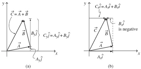
The other operation going on in Eq. 1.1 is vector addition, and you already have an idea of what that means if you recall Figure 1.5 and the process of getting from the beginning of vector \(\vec{A}\) to the end. In that process, the quantity \(A_y\hat{j}\) represented not only the number of steps you took, but also the direction in which you took them. Likewise, the quantity \(A_z\hat{k}\) represented the number of steps you took in a different direction. The fact that these two quantities include directional information means that you cannot simply add them together algebraically; you must add them “as vectors.”
式1.1で行われているもう一つの演算はベクトルの加算です。図1.5とベクトル\(\vec{A}\)の始点から終点までの過程を思い出せば、それが何を意味するのかは既にお分かりでしょう。この過程において、量\(A_y\hat{j}\)は歩数だけでなく、歩いた方向も表しています。同様に、量\(A_z\hat{k}\)は異なる方向に歩いた歩数を表しています。これら2つの量には方向情報が含まれているため、単純に代数的に加算することはできず、「ベクトルとして」加算する必要があります。

To accomplish vector addition graphically, you simply imagine moving one vector (without changing its length or direction) so that its tail is at the head of the other vector. The sum is then determined by making a new vector that begins at the start of the first vector and terminates at the end of the second vector. You can do this graphically, as in Figure 1.5(b), where the tail of vector \(A_z\hat{k}\) is placed at the head of vector \(A_y\hat{j}\), and the sum is the vector from the beginning of \(A_y\hat{j}\) to the end of \(A_z\hat{k}\) .
ベクトルの加算をグラフィカルに行うには、片方のベクトルを（長さや方向を変えずに）移動させ、その末尾がもう一方のベクトルの先頭に来るようにするだけです。そして、最初のベクトルの始点から始まり、もう一方のベクトルの終点で終わる新しいベクトルを作成することで、ベクトルの和を求めます。図1.5(b)のように、この操作をグラフィカルに行うことができます。ここでは、ベクトル \(A_z\hat{k}\) の末尾がベクトル \(A_y\hat{j}\) の始点に配置され、和は \(A_y\hat{j}\) の始点から \(A_z\hat{k}\) の終点までのベクトルになります。

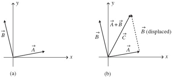
This graphical “head-to-tail” approach to vector addition works for any vectors (and any number of vectors), not just two vectors that are perpendicular to one another (as \(A_y\hat{j}\) and \(A_z\hat{k}\) were). An example of this is shown in Figure 1.8. To graphically add the two vectors \(vec{A}\) and \(\vec{B}\) in Figure 1.8(a), you simply imagine moving one of the two vectors so that its tail is at the position of the other vector's head (it doesn't matter which vector you choose to move; the result will be the same). This is illustrated in Figure 1.8(b), in which vector \(\vec{B}\) has been displaced so that its tail is at the head of vector \(\vec{A}\). The sum of these two vectors (called the “resultant” vector \(\vec{C} = \vec{A} + \vec{B}\)) is the vector that extends from the beginning of \(\vec{A}\) to the end of \(\vec{B}\).
このグラフィカルな「頭から尾まで」のベクトル加算アプローチは、互いに直交する 2 つのベクトル (\(A_y\hat{j}\) と \(A_z\hat{k}\) のように) だけでなく、任意のベクトル (および任意の数のベクトル) に機能します。 この例を図 1.8 に示します。 図 1.8(a) の 2 つのベクトル \(vec{A}\) と \(\vec{B}\) をグラフィカルに加算するには、2 つのベクトルのうちの 1 つを、その尾がもう一方のベクトルの先頭の位置にくるように移動するだけです (どちらのベクトルを移動しても結果は同じです)。 これは図 1.8(b) に示されており、ベクトル \(\vec{B}\) が、その尾がベクトル \(\vec{A}\) の先頭にくるように移動されています。これら2つのベクトルの合計（「結果」ベクトル\(\vec{C} = \vec{A} + \vec{B}\)と呼ばれる）は、\(\vec{A}\)の始めから\(\vec{B}\)の終わりまで伸びるベクトルです。

Knowing how to add vectors graphically means you can always determine the sum of two or more vectors simply using a ruler and a protractor; just draw the vectors head-to-tail (being careful to maintain each vector's length and angle), sketch the resultant from the beginning of the first to the end of the last, and then measure the length (using the ruler) and angle (using the protractor) of the resultant. This approach can be both tedious and inaccurate, so here's an alternative approach that uses the components of each vector: if vector \(\vec{C}\) is the sum of two vectors \(\vec{A}\) and \(\vec{B}\), then the magnitude of the \(x\)-component of vector \(\vec{A}\) (which is just \(C_x\)) is the sum of the magnitudes of the \(x\)-components of vectors \(\vec{A}\) and \(\vec{B}\) (that is, \(A_x + B_x\)), and the magnitude of the \(y\)-component of vector \(\vec{C}\) (called \(C_y\)) is the sum of the magnitudes of the \(y\)-components of vectors \(\vec{A}\) and \(\vec{AB}\) (that is, \(A_y + B_y\)). Thus
ベクトルを図式的に追加する方法がわかれば、定規と分度器を使用するだけで、2 つ以上のベクトルの合計をいつでも簡単に決定できます。つまり、ベクトルを頭から尾まで描き (各ベクトルの長さと角度を維持するように注意します)、最初のベクトルの始めから最後のベクトルの終わりまでの結果をスケッチし、結果の長さ (定規を使用) と角度 (分度器を使用) を測定します。このアプローチは面倒で不正確になる可能性があるため、各ベクトルの要素を使用する代替アプローチを紹介します。ベクトル \(\vec{C}\) が 2 つのベクトル \(\vec{A}\) と \(\vec{B}\) の和である場合、ベクトル \(\vec{A}\) の \(x\) 要素の大きさ (\(C_x\)) は、ベクトル \(\vec{A}\) と \(\vec{B}\) の \(x\) 要素の大きさの和 (つまり、\(A_x + B_x\)) であり、ベクトル \(\vec{C}\) の \(y\) 要素の大きさ (\(C_y\)) は、ベクトル \(\vec{A}\) の \(y\) 要素の大きさの和です。そして\(\vec{AB}\)（つまり\(A_y + B_y\)）である。したがって

\[ \begin{align} C_x &= A_x + B_x \\ \\ C_y &= A_y + B_y \end{align} \tag{1.6} \] The rationale for this is shown in Figure 1.9.
その理由は図 1.9 に示されています。

Once you have the components \(C_x\) and \(C_y\) of the resultant vector \(\vec{C}\), you can find the magnitude and direction of \(\vec{C}\) using
結果ベクトル\(\vec{C}\)の成分\(C_x\)と\(C_y\)がわかれば、\(\vec{C}\)の大きさと方向は次の式で求められる。 \[ |\vec{C}|=\sqrt{C_x^2+C_y^2} \tag{1.7} \] and
および \[ \theta = \arctan\left(\frac{C_y}{C_x}\right) \tag{1.8} \] To see how this works in practice, imagine that vector \(\vec{A}\) in Figure 1.9 is given by \(\vec{A} = 6\hat{i} + \hat{j}\) and vector \(\vec{B}\) is given by \(\vec{B} = –2\hat{i}+ 8\hat{j}\). To add these two vectors algebraically, you simply use Eqs. 1.6:
これが実際にどのように機能するかを確認するために、図1.9のベクトル\(\vec{A}\)が\(\vec{A} = 6\hat{i} + \hat{j}\)で与えられ、ベクトル\(\vec{B}\)が\(\vec{B} = –2\hat{i}+ 8\hat{j}\)で与えられていると想像してください。これらの2つのベクトルを代数的に加算するには、式1.6を使用します。

\[ C_x = A_x + B_x = 6 + (–2) = 4 \] \[ C_y = A_y + B_y = 1 + 8 = 9 \] so \(\vec{C} = 4\hat{i}+ 9\hat{j}\). If you wish to know the magnitude of \(\vec{C}\), you can just plug the components into Eq. 1.7 to get
つまり\(\vec{C} = 4\hat{i}+ 9\hat{j}\)となる。\(\vec{C}\)の大きさを知りたい場合は、式1.7に各要素を代入すれば、 \[ \begin{align} |\vec{C}| &= \sqrt{C_x^2+C_y^2}=\sqrt{4^2+9^2} \\ \\ &=\sqrt{16+81}=9.85 \end{align} \] And the angle that \(\vec{C}\) makes with the positive x-axis is given by Eq. 1.8:
そして、\(\vec{C}\)が正のx軸となす角度は式1.8で与えられます。 \[ \begin{align} \theta &= \arctan\left(\frac{C_y}{C_x}\right) \\ \\ &=\arctan\left(\frac{9}{4}\right) = 66.0^\circ \end{align} \]

With the basic operations of vector addition and multiplication of a vector by a scalar in hand, you're ready to begin thinking about the more advanced uses of vectors. But you're also ready to attack a variety of problems involving vectors, and you can find a set of such problems at the end of this chapter.⁷
ベクトルの加算とスカラー乗算という基本的な演算を習得すれば、ベクトルのより高度な利用法について考え始める準備が整います。また、ベクトルに関する様々な問題に取り組む準備も整います。本章の最後には、そのような問題集が掲載されています。⁷

⁷ Remember that full solutions are available on the book's website.
完全な解答は本のウェブサイトで入手できることを覚えておいてください。

1.5 Non-Cartesian unit vectors 非直交座標系単位ベクトル

The three straight, mutually perpendicular axes of the Cartesian coordinate system are immensely useful for a variety of problems in physics and engineering. Some problems, however, are much easier to solve in other coordinate systems, often because the axes of those systems more closely align with the directions over which one or more of the parameters relevant to the problem remain constant or vary in a predictable manner. The unit vectors of such non-Cartesian coordinate systems are the subject of this section, and transformations between coordinate systems are discussed in Chapter 4.
直交座標系の3本の互いに直交する直線軸は、物理学や工学における様々な問題に非常に有用です。しかしながら、一部の問題は他の座標系で解く方がはるかに容易です。これは多くの場合、他の座標系の軸が、問題に関連する1つ以上のパラメータが一定に保たれるか、予測可能な方法で変化する方向とより密接に一致するためです。このような非直交座標系の単位ベクトルについては本節で扱い、座標系間の変換については第4章で説明します。

As described earlier, it takes exactly N numbers to unambiguously represent any location in a space of N dimensions, which means you have to specify three numbers (such as \(x, y,\) and \(z\)) to designate a location in our Universe of three spatial dimensions. However, on the two-dimensional surface of the Earth (ignoring height variation for the moment) it takes only two numbers (latitude and longitude, for example) to designate a specific point. And one of the few benefits to living on a long, infinitely thin island is that you can set up a rendezvous using only a single number to describe the location (“I'll be waiting for you at 3.75 kilometers”).
前述のように、N次元空間内の任意の位置を一義的に表すには、ちょうどN個の数値が必要です。つまり、3次元空間の宇宙における位置を指定するには、3つの数値（\(x, y,\)、\(z\)など）を指定する必要があります。しかし、地球という2次元の表面（高度の変化は一旦無視）では、特定の点を指定するのに必要なのは2つの数値（例えば緯度と経度）だけです。そして、細長く無限に細い島に住む数少ない利点の一つは、場所を表すのにたった1つの数値（「3.75キロメートルで待っています」など）を使って待ち合わせを設定できることです。

Of course, numbers define locations only after you've defined the coordinate system that you're using. For example, do you mean 3.75 kilometers from the east end of the island or from the west end? In every space of 1, 2, 3, or more dimensions, you can devise an infinite number of coordinate systems to specify locations in that space. In each of those coordinate systems, at each location there's one direction in which one of the coordinates is increasing the fastest, and if you lay a vector with length of one unit in that direction, you've defined a coordinate unit vector for that system. So in the Cartesian coordinate system, the \(\hat{i}\) unit vector shows you the direction in which the \(x\)-coordinate increases, the \(\hat{j}\) unit vector shows you the direction in which the \(y\)-coordinate increases, and the \(\hat{k}\) unit vector shows you the direction in which the \(z\)-coordinate increases. Other coordinate systems have their own coordinate unit vectors, as well.
もちろん、数字で位置を定義するには、まず使用する座標系を定義しなければなりません。例えば、島の東端から 3.75 キロメートル、それとも西端から 3.75 キロメートルという意味でしょうか。1 次元、2 次元、3 次元、あるいはそれ以上の次元を持つあらゆる空間において、その空間内の位置を指定するための座標系を無数に考案することができます。これらの座標系では、各位置において座標が最も速く増加する方向が 1 つあり、その方向に長さ 1 単位のベクトルを置けば、その座標系の座標単位ベクトルを定義できます。つまり、直交座標系では、\(\hat{i}\) 単位ベクトルは \(x\) 座標が増加する方向を示し、\(\hat{j}\) 単位ベクトルは \(y\) 座標が増加する方向を示し、\(\hat{k}\) 単位ベクトルは \(z\) 座標が増加する方向を示します。他の座標系にも独自の座標単位ベクトルがあります。

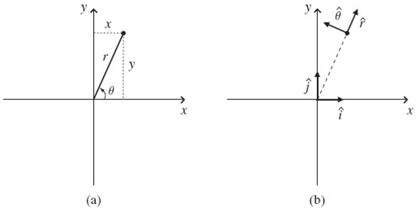
Consider the two-dimensional coordinate systems shown in Figure 1.10. In a two-dimensional space, you know that it takes two numbers to specify any location, and those numbers could be \(x\) and \(y\), defined along two straight axes that intersect at a right angle. The \(x\) value tells you how far you are to the right of the \(y\)-axis (or to the left if the \(x\) value is negative), and the \(y\) value tells you how far you are above the x-axis (or below if the y value is negative). But you could equally well specify any location in this two-dimensional space by noting how far and in what direction you've moved from the origin. In the standard version of these “polar” coordinates, the distance from the origin is called \(r\) and the direction is specified by giving the angle \(θ\) measured counterclockwise from the positive \(x\)-axis.
図 1.10 に示す 2 次元座標系を考えてみましょう。2 次元空間では、任意の位置を指定するには 2 つの数値が必要です。これらの数値は \(x\) と \(y\) で、直角に交差する 2 本の直線軸に沿って定義されます。\(x\) 値は \(y\) 軸の右側 (\(x\) 値が負の場合は左側) の距離を示し、\(y\) 値は x 軸の上側 (y 値が負の場合は下側) の距離を示します。ただし、原点からの移動距離と方向によって、この 2 次元空間内の任意の位置を指定することもできます。これらの「極」座標の標準的なバージョンでは、原点からの距離は \(r\) と呼ばれ、方向は \(x\) 軸の正方向から反時計回りに測った角度 \(θ\) で指定します。

It's easy enough to figure out one set of coordinates if you know the others; for example, if you know the values of \(x\) and \(y\), you can find r and \(θ\) using
他の座標がわかれば、1つの座標セットを求めるのは簡単です。例えば、\(x\)と\(y\)の値がわかれば、rと\(θ\)は次の式で求められます。 \[ \begin{align} r &= \sqrt{x^2+y^2} \\ \theta &= \arctan\left(\frac{y}{x}\right) \end{align} \tag{1.9} \] Likewise, if you have the values of \(r\) and \(θ\), you can find \(x\) and \(y\) using
同様に、\(r\)と\(θ\)の値がわかれば、\(x\)と\(y\)は次の式で求められます。 \[ \begin{align} x &= r \cos(θ) \\ \\ y &= r \sin(θ) \end{align} \tag{1.10} \] For the point shown in Figure 1.10, if the values of \(x\) and \(y\) are 4 cm and 9 cm, then \(r\) has a value of approximately 9.85 cm and \(θ\) has a value of 66.0°. Clearly, whether you write (\(x, y\)) = (4cm, 9cm) or (\(r, θ\)) = (9.85 cm, 66.0°), you're referring to the same location; it's not the point that's changed, it's only the point's coordinates that are different.
図1.10に示す点において、\(x\)と\(y\)の値がそれぞれ4cmと9cmの場合、\(r\)の値は約9.85cm、\(θ\)の値は66.0°になります。明らかに、(\(x, y\)) = (4cm, 9cm)と書いても、(\(r, θ\)) = (9.85 cm, 66.0°)と書いても同じ位置を指しています。点自体が変わったわけではなく、点の座標だけが異なっているのです。

And if you choose to use the polar coordinate system to represent the point, do unit vectors exist that serve the same function as \(\hat{i}\) and \(\hat{j}\) in Cartesian coordinates? They certainly do, and with a little logic you can figure out which direction they must point. After all, you know that the unit vector \(\hat{i}\) shows you the direction of increasing \(x\) and the unit vector \(\hat{j}\) shows you the direction of increasing \(y\), but now you're using \(r\) and \(θ\) instead of \(x\) and \(y\). So it seems reasonable that the unit vector \(\hat{r}\) at any location should point in the direction of increasing \(r\), and the unit vector \(\hat{\theta}\) should point in the direction of increasing \(θ\). For the point shown in Figure 1.10, that means that \(\hat{r}\) should point up and to the right, in the direction of increasing \(r\) if \(θ\) is held constant. At that same point, \(\hat{\theta}\) should point up and to the left, in the direction of increasing \(θ\) if \(r\) is held constant. These polar unit vectors are shown for one point in Figure 1.10(b).
では、点を表すのに極座標系を使うことにした場合、直交座標の \(\hat{i}\) や \(\hat{j}\) と同じ機能を果たす単位ベクトルは存在するのでしょうか？確かに存在しますし、少し論理的に考えれば、それらがどの方向を向いているのかを推測できます。結局のところ、単位ベクトル \(\hat{i}\) は \(x\) が増加する方向を示し、単位ベクトル \(\hat{j}\) は \(y\) が増加する方向を示すことはご存知でしょう。しかし、ここでは \(x\) と \(y\) の代わりに \(r\) と \(θ\) を使っています。つまり、どの位置でも単位ベクトル \(\hat{r}\) は \(r\) が増加する方向を向き、単位ベクトル \(\hat{\theta}\) は \(θ\) が増加する方向を向くのが妥当だと考えられます。図1.10に示す点の場合、\(\hat{r}\)は\(θ\)が一定であれば、\(r\)が増加する方向、つまり右上を指すことになります。同じ点において、\(\hat{\theta}\)は\(r\)が一定であれば、\(θ\)が増加する方向、つまり左上を指すことになります。これらの極座標単位ベクトルは、図1.10(b)の1点について示されています。

An important consequence of this definition is that the directions of \8\hat{r}\) and \(\hat{\theta}\) will be different at different locations. They'll always be perpendicular to one another, but they will not point in the same directions as they do for the point in Figure 1.10. The dependence of the polar unit vectors on position can be seen in the following relations:
この定義の重要な帰結は、\8\hat{r}\) と \(\hat{\theta}\) の方向が場所によって異なることです。これらは常に互いに直交しますが、図1.10の点のように同じ方向を向くことはありません。極単位ベクトルの位置依存性は、以下の関係式に示されています。 \[ \begin{align} \hat{r} &= \cos(θ)\hat{i} + \sin(θ)\hat{j} \\ \\ \hat{\theta} &= –\sin(θ)\hat{i} + \cos(θ)\hat{j} \end{align} \tag{1.11} \] So if \(θ = 0\) (which means your location is on the \(+x\)-axis), then \(\hat{r} = \hat{i}\) and \(\hat{\theta}= \hat{j}\). But if \(θ = 90°\) (so your location is on the \(+y\)-axis), then \(\hat{r}= \hat{j}\) and \(\hat{\theta}= –\hat{i}\).
したがって、\(θ = 0\)（つまり、あなたの位置は\(+x\)軸上にある）の場合、\(\hat{r} = \hat{i}\)かつ\(\hat{\theta}= \hat{j}\)となります。しかし、\(θ = 90°\)（つまり、あなたの位置は\(+y\)軸上にある）の場合、\(\hat{r}= \hat{j}\)かつ\(\hat{\theta}= –\hat{i}\)となります。

Does this dependence on position mean that these unit vectors are not “real” vectors? That depends on your definition of a real vector. If you define a vector as a quantity with magnitude and direction, the polar unit vectors do meet your definition. But they do not meet the definition of free vectors described in Section 1.1, since they may not be moved without changing their direction.
位置に依存するということは、これらの単位ベクトルが「実」ベクトルではないことを意味するのでしょうか？それは、実ベクトルの定義によって異なります。ベクトルを大きさと方向を持つ量と定義するならば、極単位ベクトルはその定義を満たします。しかし、極単位ベクトルは、方向を変えずに動かすことはできないため、第1.1節で説明した自由ベクトルの定義を満たしません。

This means that if you express a vector in polar coordinates and then take the derivative of that vector, you'll have to account for the change in the unit vectors, as well. That's one of the advantages offered by Cartesian coordinates – the unit vectors do not change no matter where you go in the space.
つまり、ベクトルを極座標で表現し、そのベクトルの微分を取る場合、単位ベクトルの変化も考慮する必要があります。これは直交座標の利点の一つです。単位ベクトルは空間のどこに移動しても変化しません。

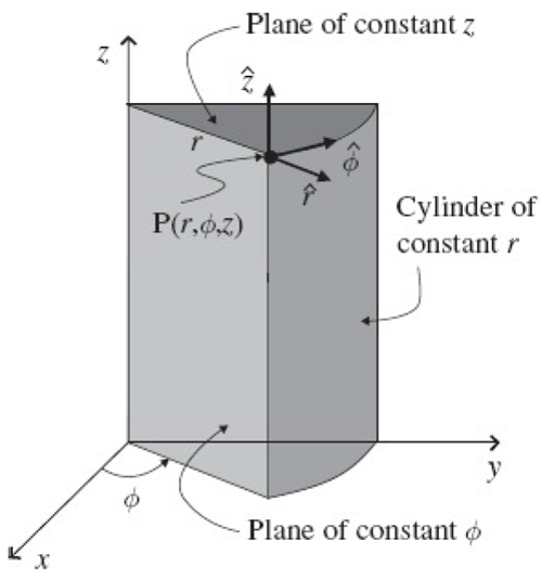
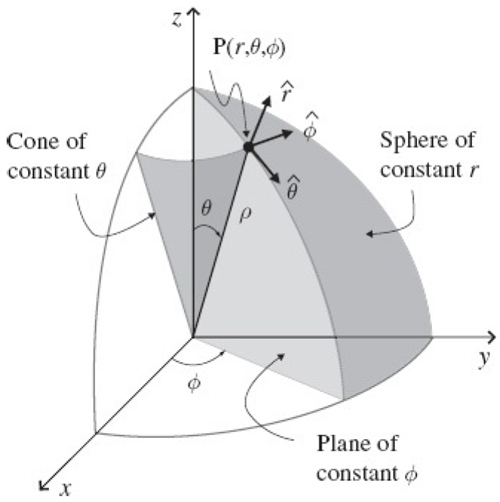
As you might expect, the situation is slightly more complicated for three- dimensional coordinate systems. Whether you choose to use Cartesian or non- Cartesian coordinates, you're going to need three variables to represent all the possible locations in a three-dimensional space, and each of the coordinates is going to come with its own unit vector. The two most common three- dimensional non-Cartesian coordinate systems are cylindrical and spherical coordinates, which you can see in Figures 1.11 and 1.12.
ご想像のとおり、3次元座標系の場合は状況が少し複雑になります。直交座標系と非直交座標系のどちらを使用するにしても、3次元空間におけるあらゆる位置を表すには3つの変数が必要になり、それぞれの座標には独自の単位ベクトルが付随します。最も一般的な3次元非直交座標系は、円筒座標系と球座標系です。これらは図1.11と図1.12に示されています。

In cylindrical coordinates a point \(P\) is specified by \(r, \phi, z\), where \(r\) (some-times called \(ρ\)) is the perpendicular distance from the \(z\)-axis, \(\phi\) is the angle measured from the \(x\)-axis to the projection of \(r\) onto the \(xy\) plane, and \(z\) is the same as the \(z\) in Cartesian coordinates. Here's how you find \(r, \phi,\) and \(z\) if you know \(x, y,\) and \(z\):
円筒座標では、点 \(P\) は \(r, \phi, z\) で指定されます。ここで、\(r\) (\(ρ\) と呼ばれることもあります) は \(z\) 軸からの垂線距離、\(\phi\) は \(x\) 軸から \(r\) を \(xy\) 平面に投影した角度、\(z\) は直交座標における \(z\) と同じです。\(x, y,\) と \(z\) がわかっている場合、\(r, \phi,\) と \(z\) を求める方法は次のとおりです。

The following equations relate the Cartesian to the cylindrical unit vectors:
次の式は、直交座標と円筒形の単位ベクトルを関連付けます。 \[ \begin{align} \hat{r} &= \cos(\phi)\hat{i}+\sin(\phi)\hat{j} \\ \\ \hat{\phi} &= -\sin(\phi)\hat{i}+\cos(\phi)\hat{j} \\ \\ \hat{z} &= \hat{z} \end{align} \tag{1.14} \]

In spherical coordinates a point \(P\) is specified by \(r, θ, \phi\) where \(r\) represents the distance from the origin, \(θ\) is the angle measured from the \(z\)-axis toward the \(xy\) plane, and \(\phi\) is the angle measured from the \(x\)-axis (or \(xz\) plane) to the constant-\(\phi\) plane containing point \(P\). With the \(z\)-axis up, \(θ\) is sometimes called the zenith angle and \(\phi\) the azimuth angle. You can determine the spherical coordinates \(r, θ,\) and \(\phi\), from \(x, y,\) and \(z\) using the following equations:
球座標では、点 \(P\) は \(r, θ, \phi\) で指定されます。ここで、\(r\) は原点からの距離、\(θ\) は \(z\) 軸から \(xy\) 平面に向かって測った角度、\(\phi\) は \(x\) 軸（または \(xz\) 平面）から点 \(P\) を含む定数 \(\phi\) 平面に向かって測った角度です。\(z\) 軸を上にした場合、\(θ\) は天頂角、\(\phi\) は方位角と呼ばれることもあります。球座標 \(r, θ,\) と \(\phi\) は、\(x, y,\) と \(z\) から次の式で決定できます。 \[ \begin{align} r &= \sqrt{x^2+y^2+z^2} \\ \\ \theta &= \arccos\left(\frac{z}{\sqrt{x^2+y^2+z^2}}\right) \\ \\ \phi &= \arctan\left(\frac{y}{x}\right) \end{align} \tag{1.15} \] And you can find \(x, y,\) and \(z\) from \(r, θ,\) and \(\phi\) using:
そして、\(r, θ,\) と \(\phi\) から \(x, y,\) と \(z\) を求めるには次のようにします。 \[ \begin{align} x &= r\sin(\theta)\cos(\phi) \\ \\ y &= r\sin(\theta)\sin(\phi) \\ \\ z &= r\cos(\theta) \end{align} \tag{1.16} \] In spherical coordinates, a vector at the point \(P\) is specified in terms of three mutually perpendicular components with unit vectors perpendicular to the sphere of radius \(r\), perpendicular to the plane through the \(z\)-axis at angle \(\phi\), and perpendicular to the cone of angle \(θ\). The unit vectors \((\hat{r},\hat{\theta},\hat{\phi})\) form a right- handed set, and are related to the Cartesian unit vectors as follows:
球座標では、点 \(P\) におけるベクトルは、半径 \(r\) の球面に垂直な単位ベクトル、角度 \(z\) 軸を通る平面に垂直な単位ベクトル、および角度 \(θ\) の円錐に垂直な単位ベクトルからなる、互いに直交する3つの成分で表されます。単位ベクトル \((\hat{r},\hat{\theta},\hat{\phi})\) は右手系の集合を形成し、直交座標系の単位ベクトルと以下のように関連しています。 \[ \begin{align} \hat{r} &= \sin(\theta)\cos(\phi)\hat{i}+\sin(\theta)\sin(\phi)\hat{j}+\cos(\theta)\hat{k} \\ \\ \hat{\theta} &= \cos(\theta)\cos(\phi)\hat{i}+\cos(\theta)\sin(\phi)\hat{j}-\sin(\theta)\hat{k}\\ \\ \hat{\phi}&=-\sin(\phi)\hat{i}+\cos(\phi)\hat{j} \end{align} \tag{1.17} \]

You may be asking yourself “Do I really need all these different unit vectors?” Well, need may be a bit strong, but your life will certainly be easier if you're trying to describe motion along a line of constant longitude on a spherical planet (the \(\hat{\theta}\) direction) or the direction of a magnetic field around a current- carrying wire (the \(\hat{\phi}\)direction). You'll find some examples of that in the problems at the end of this chapter.
「こんなにたくさんの異なる単位ベクトルが本当に必要なの？」と自問自答するかもしれません。確かに必要性は高いかもしれませんが、球状の惑星上の一定経度の線に沿った動き（\(\hat{\theta}\)方向）や、電流が流れる導線の周りの磁場の方向（\(\hat{\phi}\)方向）を記述しようとする場合、確かに作業は楽になります。この章の最後にある問題集に、その例がいくつか掲載されています。

1.6 Basis vectors 基底ベクトル

If you think about the unit vectors \(\hat{i},\hat{j},\) and \(\hat{k}\) and vector components such as \(A_x\hat{i}, A_y\hat{j},\) and \(A_z\hat{k}\), you may realize that any vector in our three-dimensional Cartesian coordinate system can be made up of three components, each one telling you how many steps to take in the direction of one of the coordinate axes. Since those steps may be large or small, in the positive or negative direction, you can reach any point in the space containing these vectors. Little wonder, then, that \(\hat{i},\hat{j},\) and \(\hat{k}\) are one example of “basis vectors” in this space; combined with appropriate magnitudes, they form the basis of any vector in the space.
単位ベクトル \(\hat{i},\hat{j},\) と \(\hat{k}\)、そして \(A_x\hat{i}, A_y\hat{j},\) と \(A_z\hat{k}\) といったベクトル成分について考えると、3次元直交座標系における任意のベクトルは3つの成分から成り、各成分はいずれかの座標軸の方向に何ステップ進むべきかを示していることがわかるでしょう。これらのステップは大きくても小さくても、正の方向でも負の方向でも構わないので、これらのベクトルを含む空間内の任意の点に到達できます。したがって、\(\hat{i},\hat{j},\) と \(\hat{k}\) がこの空間における「基底ベクトル」の一例であることは不思議ではありません。適切な大きさと組み合わせることで、これらが空間内の任意のベクトルの基底を形成します。

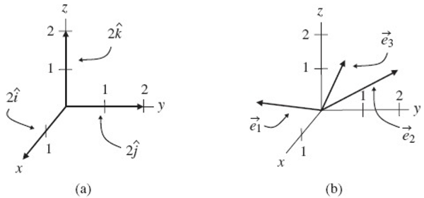
And you don't need to use only these particular vectors to make up any vector in this space – you can easily imagine using three vectors that are twice as long as the unit vectors \(\hat{i},\hat{j},\) and \(\hat{k}\), as shown in Figure 1.13(a). Although the vector components would change if you switched to these longer basis vectors, you'd have no trouble using them to make up any vector within the space. Specifically, if the unit vectors were twice as long, the values of \(A_x, A_y,\) and \(A_z\) would have to be only half as big to reach a given point in space.
また、この空間内の任意のベクトルを構成するために、これらの特定のベクトルだけを使用する必要はありません。図1.13(a)に示すように、単位ベクトル \(\hat{i},\hat{j},\) と \(\hat{k}\) の2倍の長さを持つ3つのベクトルを使用することも容易に想像できます。これらのより長い基底ベクトルに切り替えるとベクトルの成分は変化しますが、空間内の任意のベクトルを構成する際に問題なく使用できます。具体的には、単位ベクトルの長さが2倍になった場合、空間内の任意の点に到達するのに必要な \(A_x, A_y,\) と \(A_z\) の値は半分で済みます。

You might even think of using three non-orthogonal, non-unit vectors such as the vectors \(\vec{e}_1,\vec{e}_2,\) and \(\vec{e}_3\) in Figure 1.13(b) as your basis vectors. Of course, if you were to select three coplanar vectors (that is, vectors lying in the same plane), you'd quickly find that scaling and combining those vectors allows you to reach any point within that plane, but all points outside the plane would be unreachable. But as long as one of the three vectors is not coplanar with the other two, then appropriate scaling and combining will get you to any point in the space, and the vectors \(\vec{e}_1,\vec{e}_2,\) and \(\vec{e}_3\) form a perfectly usable basis set (mathematicans say that they “span” the vector space).
図 1.13(b) のベクトル \(\vec{e}_1,\vec{e}_2,\) と \(\vec{e}_3\) のような、直交しない非単位ベクトル 3 つを基底ベクトルとして使用することも考えられます。もちろん、3 つの共面ベクトル（つまり、同じ平面にあるベクトル）を選択した場合、それらのベクトルを拡大縮小して結合することでその平面内の任意の点に到達できますが、平面外のすべての点には到達できないことがすぐにわかります。ただし、3 つのベクトルのうち 1 つが他の 2 つと共面になっていない限り、適切な拡大縮小と結合によって空間内の任意の点に到達でき、ベクトル \(\vec{e}_1,\vec{e}_2,\) と \(\vec{e}_3\) は完全に使用可能な基底セットを形成します（数学者は、それらがベクトル空間を「張る」と言います）。

You can ensure that three vectors are not coplanar by requiring them to be “linearly independent,” which means that no two of the vectors may be scaled and combined to give the third, and no two are colinear (that is, lying along the same line or parallel to one another). This is often stated as the requirement that the only way to scale and combine the three vectors and get zero as the result is to scale each of the vectors by zero. In other words, for three linearly independent vectors \(\vec{e}_1,\vec{e}_2,\) and \(\vec{e}_3\), the equation
3つのベクトルが共平面でないことを保証するためには、それらのベクトルが「線形独立」である必要があります。つまり、2つのベクトルをスケールして合成しても3つ目のベクトルが得られず、2つのベクトルが共線的（つまり、同じ直線上または互いに平行）にならないということです。これは、3つのベクトルをスケールして合成し、結果として0を得る唯一の方法は、各ベクトルを0ずつスケールすることであるという要件としてよく述べられます。言い換えれば、3つの線形独立ベクトル\(\vec{e}_1,\vec{e}_2,\)と\(\vec{e}_3\)に対して、次の式が成り立ちます。 \[ A\vec{e}_1 + B\vec{e}_2 + C\vec{e}_3 = 0 \tag{1.18} \] can only be true if \(A = B = C = 0\).
\(A = B = C = 0\) の場合にのみ真となります。

So as long as you pick three linearly independent vectors, you have a viable set of basis vectors. And if you choose three non-coplanar vectors \(\vec{e}_1,\vec{e}_2,\) and \(\vec{e}_3\) of non-unit length, it's quite simple to form unit vectors from these vectors. Since dividing a vector by a positive scalar changes its length but not its direction, you simply divide each vector by its magnitude:
したがって、線形独立なベクトルを3つ選べば、有効な基底ベクトルの集合が得られます。さらに、単位長さではない共面外のベクトルを3つ（\(\vec{e}_1,\vec{e}_2,\)、\(\vec{e}_3\)）選べば、これらのベクトルから単位ベクトルを形成するのは非常に簡単です。ベクトルを正のスカラーで割ると長さは変わりますが方向は変わりませんので、各ベクトルをその大きさで割るだけで済みます。 \[ \begin{align} \hat{e}_1 &= \frac{\vec{e}_1}{|\vec{e}_1|} \\ \\ \hat{e}_2 &= \frac{\vec{e}_2}{|\vec{e}_2|} \\ \\ \hat{e}_3 &= \frac{\vec{e}_3}{|\vec{e}_3|} \end{align} \tag{1.19} \]

The concepts described in this section may be used to construct an infinite number of bases, but the most common are the “orthonormal” bases such as \(\hat{i},\hat{j},\) and \(\hat{k}\). These bases are called “ortho” because they're orthogonal (perpendicular to one another) and “normal” because they are normalized to a magnitude of one. Orthonormal bases will get you through the majority of problems you're likely to face.
このセクションで説明する概念は、無限の数の基底を構築するために使用できますが、最も一般的なのは、\(\hat{i},\hat{j},\) や \(\hat{k}\) などの「直交」基底です。これらの基底は、互いに直交（垂直）しているため「直交」、大きさが 1 に正規化されているため「正規」と呼ばれます。直交基底は、直面する可能性のあるほとんどの問題を解決できるでしょう。

One last fact about basis vectors in various coordinate systems will serve you very well if you study physics and engineering beyond the basic level, especially if your studies include the tensors discussed in Chapters 4 through 6. That fact is this: basis vectors that point along the axes of one coordinate system may be described in another coordinate system using partial derivatives.⁸ Specifically, imagine that you're converting from spherical to rectangular coordinates. The basis vector along the original spherical \((r)\) axis can be written in the Cartesian (\(x, y,\) and \(z\)) system as
様々な座標系における基底ベクトルに関する最後の事実は、物理学や工学を基礎レベルを超えて学ぶ場合、特に第4章から第6章で解説したテンソルを学習している場合、非常に役立つでしょう。それは、ある座標系の軸に沿う基底ベクトルは、偏微分を用いて別の座標系で記述できるということです⁸。具体的には、球面座標系から直交座標系に変換することを考えてみましょう。元の球面座標系の\((r)\)軸に沿う基底ベクトルは、直交座標系の(\(x, y,\)および\(z\))座標系では次のように表すことができます。

⁸ If you're not familiar with partial derivatives or need a refresher, you'll find one in the next chapter.
偏微分についてよく知らない場合や復習が必要な場合は、次の章を参照してください。

\[ \begin{align} \vec{e}_r &= \frac{\partial x}{\partial r}\hat{i}+\frac{\partial y}{\partial r}\hat{j}+\frac{\partial z}{\partial r}\hat{k} \\ \\ &=\sin\theta\cos\phi\hat{i}+\sin\theta\sin\phi\hat{j}+\cos\theta\hat{k} \end{align} \] Likewise, the \(\vec{e}_θ\) and \(\vec{e}_\phi\) basis vectors can be written as
同様に、\(\vec{e}_θ\)と\(\vec{e}_\phi\)基底ベクトルは次のように書けます。 \[ \begin{align} \vec{e}_\theta &= \frac{\partial x}{\partial \theta}\hat{i}+\frac{\partial y}{\partial \theta}\hat{j}+\frac{\partial z}{\partial \theta}\hat{k} \\ \\ &= r\cos\theta\cos\phi\hat{i}+r\cos\theta\sin\phi\hat{j}-r\sin\theta\hat{k} \\ \\ \vec{e}_\phi &= \frac{\partial x}{\partial \phi}\hat{i}+\frac{\partial y}{\partial \phi}\hat{j}+\frac{\partial z}{\partial \phi}\hat{k} \\ \\ &= -r\sin\theta\sin\phi\hat{i}+r\sin\theta\cos\phi\hat{j} \end{align} \] Notice that these basis vectors are not all unit vectors (because their magnitudes are not all equal to one), nor do they all have the same dimensions (\(\vec{e}_r\) is dimensionless, but \(\vec{e}_θ\) and \(\vec{e}_\phi\) have dimensions of length). Neither of these characteristics disqualifies these as basis vectors, and you can always turn them into unit vectors by dividing by their magnitudes (take a look at the problems at the end of this chapter and their on-line solutions if you want to see how this works).
これらの基底ベクトルはすべて単位ベクトルではないことに注意してください（大きさがすべて1ではないため）。また、すべてが同じ次元を持つわけでもありません（\(\vec{e}_r\) は無次元ですが、\(\vec{e}_θ\) と \(\vec{e}_\phi\) は長さの次元を持ちます）。これらの特徴はいずれも基底ベクトルとしての資格を失わせるものではなく、大きさで割ることでいつでも単位ベクトルに変換できます（この仕組みを知りたい場合は、この章の最後にある問題とそのオンライン解答をご覧ください）。

In general, if the coordinates of the original system are called \(x_1, x_2,\) and \(x_3\) (these were \(r, θ,\) and \(\phi\) in the example just discussed), and the coordinates of the new system are called \(x_1^\prime, x_2^\prime,\) and \(x_3^\prime\) (these were \(x, y,\) and \(z\) in the example), then the basis vectors along the original coordinate axes can be written in the new system as
一般に、元の座標系の座標を\(x_1, x_2,\)と\(x_3\)（先ほどの例では\(r, θ,\)と\(\phi\)）とし、新しい座標系の座標を\(x_1^\prime, x_2^\prime,\)と\(x_3^\prime\)（先ほどの例では\(x, y,\)と\(z\)）とすると、元の座標軸に沿った基底ベクトルは新しい座標系では次のように表すことができます。 \[ \begin{align} \vec{e}_1 &= \frac{\partial x_1^\prime}{\partial x_1}\vec{e}_1^\prime+\frac{\partial x_2}{\partial x_1}\vec{e}_2^\prime+\frac{\partial x_3^\prime}{\partial x_1}\vec{e}_3^\prime \\ \\ \vec{e}_2 &= \frac{\partial x_1^\prime}{\partial x_2}\vec{e}_1^\prime+\frac{\partial x_2}{\partial x_2}\vec{e}_2^\prime+\frac{\partial x_3^\prime}{\partial x_2}\vec{e}_3^\prime \\ \\ \vec{e}_1 &= \frac{\partial x_1^\prime}{\partial x_3}\vec{e}_1^\prime+\frac{\partial x_2}{\partial x_3}\vec{e}_2^\prime+\frac{\partial x_3^\prime}{\partial x_3}\vec{e}_3^\prime \\ \end{align} \tag{1.20} \] In other words, the partial derivatives \(\frac{x_1^\prime}{\partial x_1}\vec{e}_1^\prime,\frac{\partial x_2^\prime}{\partial x_1}\vec{e}_2^\prime,\) and \(\frac{\partial x_3^\prime}{\partial x_1}\vec{e}_3^\prime\) are the components of the first original (unprimed) basis vector expressed in the new (primed) coordinate system. For this reason, you'll find that some authors define basis vectors in terms of partial derivatives.
言い換えれば、偏微分 \(\frac{x_1^\prime}{\partial x_1}\vec{e}_1^\prime,\frac{\partial x_2^\prime}{\partial x_1}\vec{e}_2^\prime,\) と \(\frac{\partial x_3^\prime}{\partial x_1}\vec{e}_3^\prime\) は、新しい（プライム付き）座標系で表現された、最初の元の（プライムなし）基底ベクトルの要素です。このため、偏微分を用いて基底ベクトルを定義する著者もいます。

These relationships will prove to be extremely valuable in the study of coordinate-system transformation and tensor analysis, so file them away if your studies include those topics.
これらの関係は、座標系の変換やテンソル解析の研究において非常に価値があることが証明されるので、研究にこれらのトピックが含まれる場合は保存しておいてください。

1.7 Chapter 1 problems 1章の問題